Wikipedia credits C.S. Peirce as being one of the founders of statistics and specifically calls out the “Illustrations of the Logic of Science” essays. “The Probability of Induction,” published April 1878, shows Peirce groping toward the idea of confidence intervals (a term he would later coin, but hasn’t yet). He also defends Venn’s frequentist interpretation of probability by showing that the dominant subjectivist interpretation and methods lead to absurdity.
Because Peirce and others were still formulating both the terminology and conceptual underpinnings of frequentist statistics, the essay benefits (I hope) from my cover band approach. In my version, I’ll drop some of the digressions that Peirce is so overly fond of. (Let’s just say that, in general, my covers will omit Peirce’s drum solos.)
TL;DR
-
Analytical reasoning releases truths that are in some sense contained in the premises. Synthetic reasoning constructs and justifies new truths.
-
When synthetic reasoning produces quantitative estimates, you really need two numbers: the estimate and your confidence in the estimate. A procedure for estimating the latter is provided.
-
Venn’s definition of probability as the ratio of desirable results to total trials is the new kid on the block. The traditional definition tries to turn subjective degrees of belief into objective numbers. That’s a bad idea because it produces certain absurdities.
-
The root error is that subjectivist interpretations are trying to apply analytical methods to problems of synthesis.
-
A better way to operationalize belief is to treat it as the logarithm of the ratio of desirable to undesirable results. That has mathematical properties that better fit our intuitions about beliefs.
Brian’s Disclaimer
I took statistics and probability in college, but have used them very little since. I’m a symbol guy, not a numbers guy. When I worked on the Unix kernel in the early 1980s, it contained exactly one floating point number.
I. Types of inference
Consider the following syllogism:
- All Cretans are liars.
- Epimenides is a Cretan.
- Therefore, Epimenides is a liar.
This is an example of deductive reasoning, also called explicative or analytic reasoning. The latter two are the more useful terms. Explicative suggests that the syllogism is a rule of inference that exists to explain why Epimenides is a liar. Analytic comes from the Green analyein, meaning “to unloose, release, set free.” The fact that Epimenides is a liar is, in a sense, hidden within the major premise (“All Cretans are…") and the minor premise (“Epimenides is…"), and the form of the syllogism unleashes it.
The following syllogism is also analytic:
- Ninety-nine Cretans in a hundred are liars.
- Epimenides is a Cretan.
- Therefore, Epimenides is a liar.
However, the conclusion is not certain. Following Mr. Venn, we want to say that the meaning of the conclusion is that if we were to run an unbounded number of trials, 99% of them would show Epimenides is a liar. Alternately, as the number of trials grew, the fraction of the trials where Epimenides is a liar would converge to 99 out of 100.
But as with Fateful Fatima in the last essay, we only get one trial in this world. Epimenides is either a liar or he isn’t. We can finesse that by considering there to be an unlimited number of universes. In 99% of them Epimenides will be a liar.
However, we live in this universe, so it’s not clear what the point of that would be.
For purposes of scientific inquiry, what’s frequently called amplificative or synthetic reasoning is more appropriate. That last is from the Greek syntithenai, “to put together.” Rather than a hidden claim being unleashed, a new conclusion is assembled. Here’s an example:
- Minos, Sarpedon, Rhadamanthus, Deucalion, and Epimenides are all the Cretans I can think of;
- But these were all atrocious liars,
- Therefore, pretty much all Cretans must have been liars.
We’ll be working on inductive reasoning, a kind of synthetic reasoning that tries to quantify “pretty much.“ Peirce has some important qualifications in his understanding of induction, derived from his experience as a working scientist, that will appear in his later work. If you want to peek ahead, I recommend Deborah G. Mayo, “Peircean Induction and the Error-Correcting Thesis,” Transactions of the Charles S. Peirce Society, Spring, 2005, Vol. 41, No. 2, pp. 299-319.
II. The two numbers for induction
A first step in induction is just counting. For example, in the 1870 census, around 1,000,000 White children under the age of one were counted. Of them, the proportion of males was 0.5082. Around 150,000 black children were surveyed; 0.4977 were male. Does this signify a real difference between the races or just random chance?
Let’s suppose that the two races are not different and that the correct proportion of boys and girls, in both races, is 1:1. The term, and perhaps the concept of, “null hypothesis” did not exist in Peirce’s time. See “Milk, Tea, and Statistics: The Birth of Hypothesis Testing.” What would we then expect to see if large numbers of children were surveyed? What are the chances we’d get these different results?
Mathematicians have a formula for that. I won’t explain the derivation, which puts you in the position of last essay’s Bob the layperson listening to Alice the mathematician make a claim he cannot check. I hope you believe me!
The core of the formula is this calculation:
For notation, I’m using the Ruby programming language because that’s what I used to do the math. Math.sqrt is the calculation normally represented by the square root symbol, √. Multiplication is indicated by the asterisk, *, rather than a multiplication sign, ×. You can find the source here.
unadjusted_error = Math.sqrt(2*p*(1-p) / s)
unadjusted_error means that if the true probability is p (here, 0.5), and s is the number of samples taken to form our estimated probability, we may expect the difference between the measured and assumed probabilities to be kinda-sorta less than unadjusted_error. (I’ll explain the “kinda sorta” bit shortly.)
The unadjusted error for the 1,000,000 White children is this: 1_000_000 is just Ruby’s easier-to-read notation for 1000000. In the paper, Peirce uses 2_000_000 instead of 1_000_000. I think that’s an error, caused by him forgetting that 1_000_000 was the total number of children, not the number of boys. The number he arrives at seems consistent with his using 1_000_000 in the actual calculation. (Because he’s doing the math by hand and approximating, his result varies from Ruby’s.)
Math.sqrt(2*1/2*(1-1/2) / 1_000_000) # or
Math.sqrt(0.5 / 1_000_000) = 0.0007  # approximately
And for Black children:
Math.sqrt(0.5 / 150_000) = 0.002 # approximately
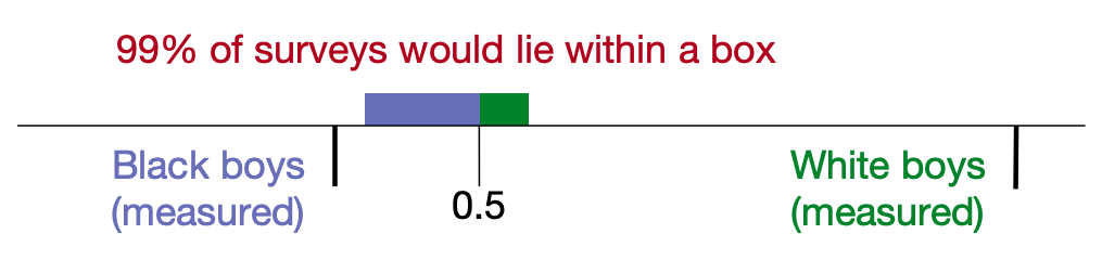
If we plot the values on a scale, we find that the measured proportions of boys lies well outside the unadjusted error. Note that the allowable error for White boys is smaller because the sample size is so much bigger.

However, we’re missing a number. If you flip 10 coins, you’d expect around five to be heads. But you wouldn’t be shocked if seven or even eight were heads. You’d even concede that if you tried it enough times you might get ten heads from ten flips. And the same is true of 20 heads, but is considerably less likely. So we don’t want an unadjusted error value. Instead, we want to know the range in which 9 out of 10, or 99 out of 100, or 9999 out of 10000 estimates would be expected to lie. That requires an adjustment of the unadjusted error. Here are some adjustments.
How often will the measured value be within X of the true value?
| one out of two times | 0.477 × unadjusted |
| 9 times out of 10 | 1.163 × unadjusted |
| 99 times out of 100 | 1.821 × unadjusted |
| 999 times out of 1000 | 2.328 × unadjusted |
| 9,999 times out of 10,000 | 2.751 × unadjusted |
| 9,999,999,999 times out of 10,000,000,000 | 4.77 × unadjusted |
For Black boys, how often would we expect a measured value to be within the spread starting at 0.5 - (1.82 * 0.002) / 2 = 0.4983? 99 times out of 100. But the measured value of 0.4977 is below that. It seems pretty unlikely the true value is 0.5.
The situation for White boys is even worse because of the larger sample size. A number as large as the measured 0.5082 would happen less often than one time out of ten billion.
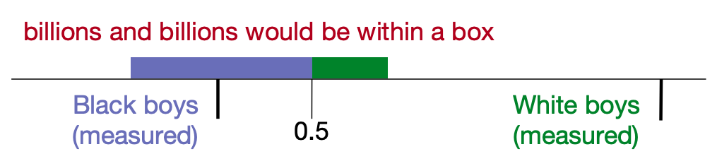
We should accept that the proportions are different for Black and White children. Neither matches the theoretical 0.5. Worldwide, male births outnumber female births, with some variation between countries. The 1870 US census’s estimate for White boys is a little below later US surveys. The ratio for Black boys is way low.
III. The conceptualist interpretation of probability
Mr. Venn’s materialist interpretation of a probability as the number of favored cases to total cases is not yet the most popular. More popular is the view espoused by Mr. De Morgan in his 1847 Formal Logic, or the Calculus of Inference, Necessary and Probable or in the recently departed Mr. Quételet’s Lettres sur la théorie des probabilités. Mr. Venn calls theirs the conceptualist view. Nowadays it’s more often called a subjectivist, personalist, or Bayesian interpretation. (Some sources cite Peirce as an early worker in Bayesian statistics, but I don’t see that in this essay.) In a conceptualist view, probability is identified as “the degree of belief that ought to attach to a proposition.” Since our first essay was on belief, we should discuss conceptual probability.
The two interpretations lead to the same actions in most situations. For those cases, we can say – by the pragmatic maxim – that they mean the same things. Still, I will now lay out problems with the conceptualist view, then discuss how we might nevertheless reasonably associate probability with the strength of belief.
Probability of what?
Our approach to probability is that it is attached to an inference rule, not to what is inferred. Consider again the case of mathematician Alice explaining a mathematical truth to non-mathematician Bob. We are interested in the probability that someone following the inference rule just believe the mathematician will result in non-mathematicians coming to correctly believe in a mathematical truth.
The conceptualist is interested in how often non-mathematicians will believe a mathematical truth independent of the reasoning process. Alternately, the conceptualist is interested in how often a desired result will occur, regardless of the cause.
This makes conceptualist probability a poor fit for logic, which is all about valid reasoning from known facts or premises.
Belief in the unknown
Suppose we have a large bag of white and black beads. Someone takes one out and hides it under a thimble. How strong is our belief that the bead, when revealed, will be black?
Last essay, we saw that the materialist gives the probability as undefined, since the ratio of favorable (black) trials to all trials is 0/0.
However, De Morgan instructs us that our belief that the bead is black has probability 0.5 because we will be equally surprised whichever color is revealed when the thimble is lifted. (“Perfect indecision, belief inclining neither way, an even chance.” – Formal Logic, 1847, p. 182.) Alternately, the strength of our belief that the bead will be white is exactly balanced by our belief that it will be black.

The absurdity of this can be seen by asking a different question: “what is the hair color of the inhabitants of Saturn?“
Another thing it’s amazing they didn’t know in 1878. To answer this, consider a color wheel like the one on the right, where all the colors shade imperceptibly into one another.

Draw a line around an arbitrary area in the chart. Do we believe Saturnian hair color is one of the colors enclosed? Since we have no evidence, the probability – according to the conceptualist view – is 1/2.

The same must be true of any other area. But that can’t be right. If two enclosed areas have probabilities of 1/2, an area that contains both of them must have a probability of at least 1, which is absurd. (See here for the rules for adding probabilities.)
A tendency toward equal probabilities
The idea that non-belief is a probability of 1/2 leads to a bias that, for any given problem, all possibilities are equally probable until we have sufficient evidence to change our belief. So consider the problem of determining the ratio of white to black beads in a vat. A conceptual point of view is that there are many equally probable possibilities:
- a vat with all black beads
- a vat with black beads except for one white bead.
- … except for two white beads.
- …
- a vat with all white beads except for one black bead.
- a vat with all white beads.
The problem of finding the probability of a drawn bead being black is identical to the problem of coming to believe which of the hypothetical urns has the same proportion of beads as the real one.
But is this a useful way of looking at probability?
Belief in belief
It is not. An example from Quételet in his Théorie des probabilités illustrates this. Suppose there is a person who knows nothing of the ocean. They are asked whether they believe that the level of the ocean rises twice daily. Unless they are allowed to reason a priori (which would surely cause them to assign a probability of zero or near zero: after all, what possible force could raise an entire ocean?), they are compelled to give a probability of 1/2.
Transported to the seacoast for m days, they can observe the tide happens every day. Therefore, their belief can be calculated as (1+m)/(2+m). (This combines conceptual presuppositions and the materialist approach to calculation, a common move by conceptualists.)
The result is not that different (in this case) from what a materialist would calculate, but it’s missing one of the two numbers from section II. There, we could say that believing the actual proportion of white boys to white girls is 50/50 would require that the 1870 census just so happened to collect numbers we’d expect to see less than one time in ten billion surveys of one million children. So we reject the 1:1 hypothesis, instead coming to believe the true ratio is closer to 0.5082 than to 0.5.
Approaches like Quételet’s leave us unable to draw such conclusions.
The big picture
The deeper problem with Quételet and company’s approach is that they are analysing induction, a synthetic procedure, as if it were analytical. They’re acting as if accumulating evidence forces discovery of a truth hidden in the facts of observation when it is better treated as supporting, with some degree of confidence, a new truth hypothesized in a free and creative act. The last essay in this series will tie together the three distinct types of logic used in scientific reasoning: abduction (hypothesis generation), deduction, and induction.
IV. Chance and belief
Probability, we’ve seen, makes an uneasy fit with belief. Better than probability is a related notion, which I’ll label chance. Here’s the difference:
The probability of something is the number of matching occurrences divided by the total number of occurrences. Chance is defined as having the same numerator but dividing it by the number of mismatches. If three trials leads to only one match, the probability is 1/3 and the corresponding chance is 1/2.
Rather than saying belief is probability, let’s say that belief is as the logarithm of chance. Nowadays, this function is known as the logit or log-odds function. According to Ian Hacking, Peirce pioneered it. (Ian Hacking, The Taming of Chance, Cambridge University Press, 1990, p. 211.) Here are the benefits:
First, rather than representing the lack of opinion as a 1/2 probability, it’s a 1/1=1 chance. And the logarithm of 1 is 0, which nicely stands for no belief. When the chance goes below 1, the logarithm goes negative, which nicely represents disbelief.
Second, probabilities have an upper bound of 1.0, but chances have no upper bound. Therefore belief (the logarithm of chance) has no upper bound. It makes sense that, as the chance of a favorable outcome increases smoothly toward infinity, our belief should as well.
Third, consider the case where the probability of one reasoning procedure producing a correct answer is 0.8 and the probability of a second is 0.9. In a given situation, both apply. They may either agree or disagree. But if they agree, it seems intuitive that our belief in the combination should be greater than would be our belief in either alone. Let’s work out the numbers, starting with the rule that independent probabilities are multiplied: Peirce gave the rules for combining probabilities in both this essay and the previous one, but I didn’t transliterate those sections. They’re the same as you probably learned in secondary school or college. The presentation is slightly different, due to his emphasis on the probabilities of inferences rather than events. If interested, see my separate coverage of that part of this essay.
| both answer correctly | 0.8 × 0.9 = 0.72 |
| first is incorrect and second is correct | 0.2 × 0.9 = 0.18 |
| first is correct and second is incorrect | 0.8 × 0.1 = 0.08 |
| both answer incorrectly | 0.2 × 0.1 = 0.02 |
What is the chance of them both agreeing and being correct (vs. both agreeing and being incorrect)? (0.72 / 0.02) = 36.
How can that be calculated using chances from the very beginning? The chance of answering correctly using the first procedure is
0.8 / 0.2 = 4. The chance using the second is 0.9 / 0.1 = 9. So the chance of both being correct is 4 * 9 = 36.
This is easier to see if you write out and transform fractions, but I’ve so far balked at learning to use MathJax so that I can put pretty equations in blog posts. Multiplication can be done by the addition of logarithms, which is why slide rules are so handy. So we can say that our belief is 1.4 in the first procedure, 2.2 in the second, and 3.6 for their combination. The idea of independent inferences combining beliefs additively makes sense.
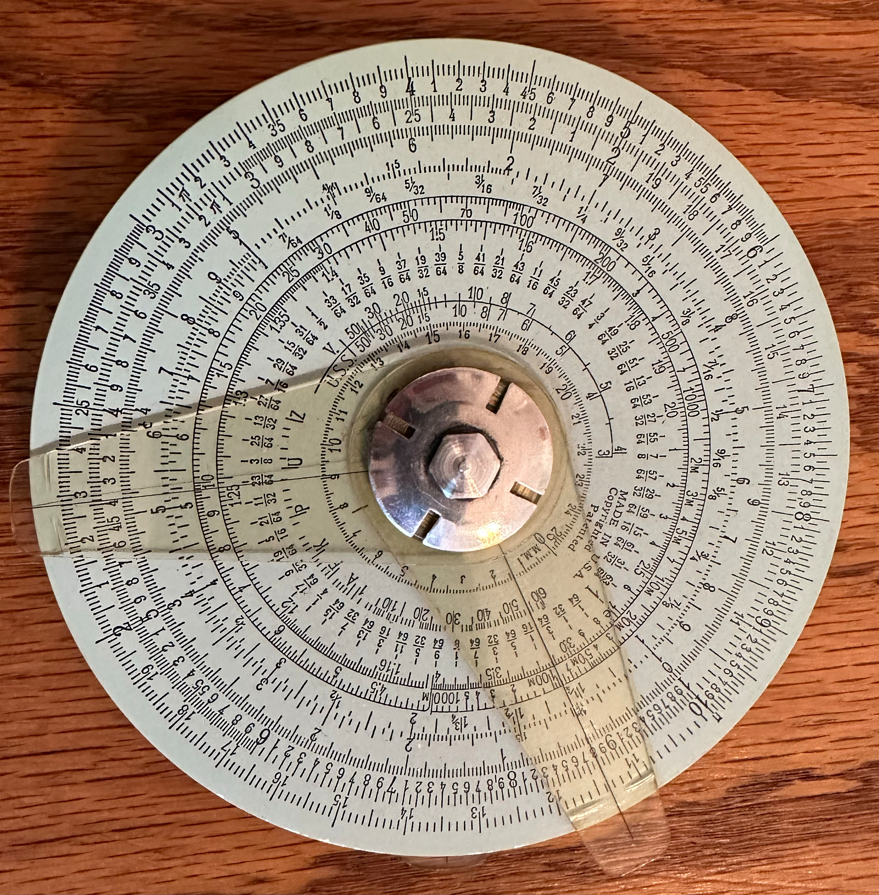 My childhood slide rule.
Fourth, while belief isn’t only an emotion, it is an emotion. As such, it falls under the category of sensations (belief is the perception of an internal state of your mind). Fechner’s psycho-physical law is an experimental result that the intensity of a sensation is proportional to the logarithm of the external force that causes it. So it makes sense to treat beliefs the same way.
Liner notes for the 2026 reissue
-
It’s worth noting that Peirce will, in about 20 years, abandon the frequentist interpretation of probability for what’s now called a propensity interpretation. In that interpretation, probability is a real thing that is inherent in objects in the world, like dice. I don’t know what the practical implications of that are (yet), but it supports his later evolutionary cosmology, wherein entities develop “habits” that reduce their propensity to respond with randomness.
In the meantime, he attaches probability to process: “In the case of synthetic inferences we only know the degree of trustworthiness of our proceeding[s].” “All human certainty consists merely in our knowing that the processes by which our knowledge has been derived are such as must generally have led to true conclusions.”
-
Peirce ends the essay by returning to his theme that the truth will be found via the long-run consensus of those who inquire after it. The way repeated observations narrow the error bounds around an estimated probability reminds him of that. “That the rule of induction will hold good in the long run may be deduced from the principle that reality is only the object of the final opinion to which sufficient investigation would lead.”
-
I noticed that his method of calculating error ranges doesn’t produce good results for his second Cretan Liars example. His syllogism starts by listing five Cretans who are liars, then concludes that “pretty much all Cretans must have been liars.” But if we then conclude that the “null hypothesis” is that Cretans are liars with probability 1.0 – the same as the measured estimate – the formula for
unadjusted_errorgives a range of size 0. That seems wrong. Things are better if the null hypothesis is that Cretans are actually liars with probability 1/2, so it seems that picking the assumed probability is both important and weakly motivated. Perhaps this is what leads Peirce to work on Bayesian statistics.